¶ Contents
¶ Excel
¶ Formatting
¶ Shade Rows where column contains duplicates
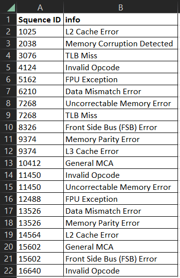
Before
- Select range
- Select "Conditional Formatting"
- Select "New Rule"
- Select "Use a formula to determine which cells to format"
- Enter the formula
=COUNTIF($A$2:$A2,$A2)>1 - Set up formatting style and click OK
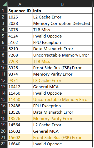
After
¶ Shade Alternate Rows
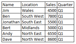
Before
- Select range
- Select "Conditional Formatting"
- Select "New Rule"
- Select "Use a formula to determine which cells to format"
- Enter the formula
=MOD(ROW(),2) - Select a formattings style and click OK
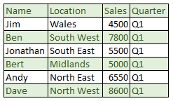
After
This same trick works on OpenOffice, though it should be noted that the seperator is not , but is ;
¶ Shade Row Based on value
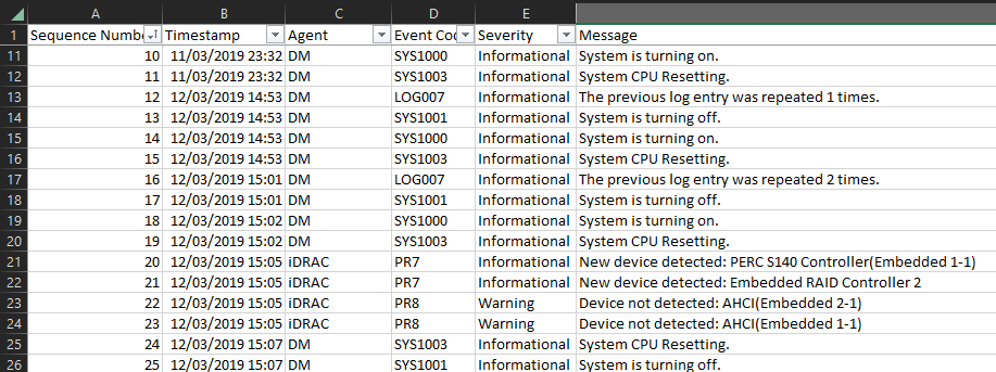
before
- Select range
- Select "Conditional Formatting"
- Select "New Rule"
- Select "Use a formla to determine which cells to format"
- Enter the forumula
=$E2="Warning" - Set the formatting and click OK
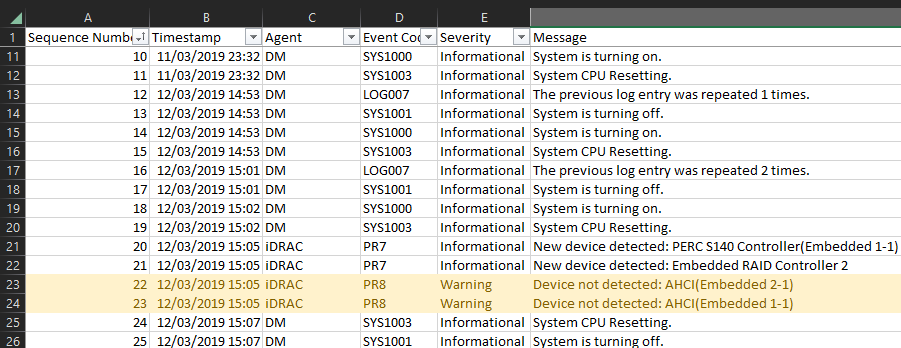
after
¶ Functions and Formulae
¶ Find unique values using a formula
To return unique values from a range, use the "UNIQUE" formula.
If there is more than one result, this will result in a "spill" condition. This means that the results will spill in to the cells below. Because of this, it is not supported in tables.
=UNIQUE(array, [by_col], [exactly_once])
Arguments in square brackets ([ ]) are optional
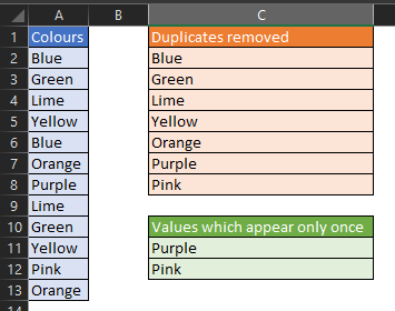
Example: You have a list of colours and want to remove the duplicates.
In cell C1, you would enter the following
=UNIQUE(A2:A13)
Further to this, you wish to exclude the values which appear only once and ignore duplicated values. In cell C10, you would enter:
=UNIQUE(A2:A13,FALSE,TRUE)
It may also be that the range you use is variable and may contain blanks. If you wish to ignore these (they will be returned as a '0'), then you can use the following:
=UNIQUE(FILTER(RANGE,RANGE<>"")
¶ Count unique values
Example
| A | B | C | D | E | |
|---|---|---|---|---|---|
| 1 | 546 | Unique values | 3 | ||
| 2 | 654 | ||||
| 3 | 456 | ||||
| 4 | 546 | ||||
| 5 | 546 | ||||
| 6 | 546 | ||||
| 7 | 456 | ||||
| 8 | 654 | ||||
| 9 | 456 | ||||
| 10 | 654 |
In order to count the unique values, an 'array' formula needs to be used. In cell 'E1', enter the following
=SUM(1/COUNTIF(A1:A10,A1:A10))
Once keyed in, you must press Ctrl+Shift+Enter
¶ COUNTIF with more than one value
On certain occasions you may want to count values depending on another condition. For this you can use COUNTIF(range, criteria). This works well when you have a single criteria to check against. On occasion you may wish to count items depending on more than one value. For this, you will need to use a combination of formulae.
| A | B | |
|---|---|---|
| 1 | Case Number | Status |
| 2 | 34567765 | Open |
| 3 | 45678765 | Closed |
| 4 | 23454533 | Closed |
| 5 | 98765671 | Pending |
| 6 | 56776542 | Closed |
In the simple example above, you may want to know how many cases are 'Closed' and 'Pending'. In this example its quite easy for us to count the different status and add them up. However in a larger dataset, you'll probably want computer to do the work.
For this, we can use a combination of SUM and COUNTIF like this:
=SUM(COUNTIF(B2:B6, {"Closed", "Pending"}))
This should give the answer 4.
If you do not use the SUM part of the forumula, you will have a "spill" answer and you will receive two values (one for "Closed" and one for "Pending, 3 and 1 respectively)
¶ Convert Base
Convert from base36 to decimal
=DECIMAL(A1,36)
| A | B | C | D | E | |
|---|---|---|---|---|---|
| 1 | 6T2YF42 | Decimal | 14819178242 |
Convert from decimal to base36
=BASE(A1,36)
| A | B | C | D | E | |
|---|---|---|---|---|---|
| 1 | 14819178242 | Base36 | 6T2YF42 |
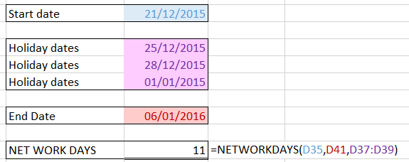
¶ Working days between two dates (including holidays)
¶ Find and Replace
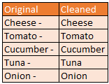
This can be done using the find and replace feature in Excel, but can also be done using a formula; SUBSTITUTE(text, old-text, new-text) function, you can find text in a string and have it replaced. Example below:
=SUBSTITUTE(A2, " - ", "")
¶ Index Match
Powerful combination of functions to find and return values in a spreadsheet.
=INDEX(array, row_number)
=MATCH(lookup_value, lookup_array, [match_type])
For INDEX/MATCH, these will be combined thusly:
=INDEX(array, MATCH(lookup_value, lookup_array, [match_type])) - in this way the MATCH function is used to find the row number to extract. This then means that the INDEX function can return that row from the array.
The below table shows a list of people and what their top seller was for each month.
| A | B | C | D | E | F | |
|---|---|---|---|---|---|---|
| 1 | Jan | Feb | Mar | Apr | June | |
| 2 | Jim | Apples | Oranges | Bananas | Apples | Apples |
| 3 | Erica | Apples | Bananas | Bananas | Apples | Oranges |
| 4 | Julia | Oranges | Oranges | Apples | Apples | Apples |
| 5 | Ethan | Apples | Apples | Apples | Apples | Bananas |
| 6 | Brian | Oranges | Apples | Bananas | Bananas | Apples |
| 7 | ||||||
| 8 |
Let us say we want to quickly find out what Erica's top seller was for March.
First we need to understand which row Erica is in.
=MATCH(B3,B2:B6,0) this should resolve to 2 as 'Erica' is in the second row of the array (cell B3 = "Erica"). The 0 at end specifies the match type; 0 forces an exact match.
The row number is relative to the array, not to the sheet; Erica is in the 3rd row of the sheet but the 2nd row of the array specified.
I would recommend using0as the match type to force exact matches only otherwise unexpected and undesirable results will be returned.
We can now feed that output in to the INDEX function:
=INDEX(D2:D6,2) This will look up the 2nd row in that array and will return "Bananas".
Now we can combine the two functions in to a forumula:
=INDEX(D2:D6,MATCH(B3,B2:B6,0))
This will also return "Bananas"
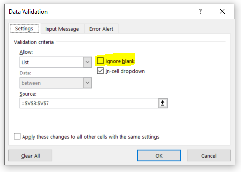
¶ Drop down list (with blanks)
- Create a list of valid entries
- Select cell (or cells) to have drop down option
- Select "Data" on the ribbon UI
- Select "Data Validation"
- Select "List" under the 'Allow' section
- Enter or select source in the 'Source' box
- If you want to have a blank option in the list, ensure your source data has a blank line and uncheck "Ignore blank" next to the 'Allow' section
¶ Keyboard Shortcuts
| key combination | action |
|---|---|
| Ctrl + Shift + L | Add filtering |
| Ctrl + Shift + + | Insert row, column, cell |
¶ Word
¶ Linking within document
- Add book mark
- Select text to be the bookmark/anchor
- Go to "Insert" on ribbon
- Select "Bookmark"
- Enter details (Note: The bookmark name cannot have any spaces in it)
- Select the text to link from
- Right click and select "Link"
- Select "Place in This Document" under "Link to:"
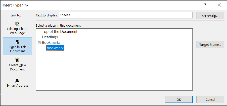
- Select the appropriate bookmark or heading to link to